Simulating with the 3Di Modeller Interface

This section explains the available options for running simulations in the 3Di Modeller Interface.

Starting a simulation

1. Open the 3Di Modeller Interface

2. Activate the ‘3Di Models and Simulation panel’ by clicking on the pictogram () in the toolbar.

3. Click on the ‘Simulate’ icon.

4. Click on ‘New Simulation’.

5. Select the model you want to simulate. If you have access to more than one organisation, choose the organisation that billing should go to. Then click on ‘Next’.

6. A panel with different scenario options will now appear, check the options you want to be used in the calculations of your simulation:

   • Initial condition

     • Initial conditions: To define the use of initial water levels in 1D, 2D or Ground water or a (previously) saved state.

   • Forcings

     • Boundary conditions: Boundary conditions are taken from the spatialite directly.

     • Laterals: Select laterals to use in the model.

     • Dry weather flow: Include dry weather flow in your model.

     • Precipitation: Define precipitation in the model.

     • Wind: Define wind in the model.

     • Raster edits

     • Leakage

     • Sources and sinks

     • Local or time series rain

     • Obstacle edits

   • Events

     • Structure controls: Modify hydraulic structure parameters.

     • Breaches: To select a breach to open in the model.

   • Other options

     • Generate saved state after simulation: To save the end result of the simulation as a saved state.

     • Post-processing in Lizard: This is a feature that is only available for users of organisations that have a Lizard account. It enables you to store the results in the cloud and it triggers automated post-processing of water depth, water levels, time of arrival, flood hazard rating and damage estimations maps.

     • Multiple simulations (becomes available when using either breaches or precipitation): To define multiple simulations with rainfall or breaches. Useful when simulating multiple events on the same model.

7. Name the simulation. Users within your organisation will be able to find this simulation and its results based on the name. Adding ‘Tags’ can clarify for other users what your simulation calculated or can be used to assign a simulation a certain project name or number.

8. Set the ‘Duration’ of the simulation. Optionally, you can specify the time zone for the simulation duration. This is especially relevant if you use radar rain in your simulation that is also defined in a specific time zone.

9. The next steps depend on the selection of options from the initial screen of the wizard (step 6). Unchecked options will be omitted by the wizard. The different options are explained below.

10. If you want, change the Simulation settings. The setting values that are shown are the ones you have specified in the schematisation spatialite. This page in the simulation wizard allows you to override specific settings for this specific simulation. This does not change the values of the simulation settings in the spatialite.

11. Click Add to queue to start the simulation.

You can follow the progress of your simulation by clicking on the Simulate icon in the 3Di Models and Simulations panel. You can also terminate your simulation by clicking on ‘Stop Simulation’.

Once the simulation is done the results will be available for 7 days. For information on how to download, view and analyze results, see Analysing results in the 3Di Modeller Interface.

Note

If you want to remove a simulation from the queue before it has started, use the Live status page on 3Di Management.

Substances

When using the water quality module, you define the substances to be used on the substances page. Each substance must have a unique name. Specifying the units is optional; units can be any text, with a max length of 16 characters.

Boundary conditions

• From simulation template: If the 3Di model contains boundary conditions, a timeseries for each boundary condition will be included in the simulation template.

• Upload files(s): You can upload CSV files to replace the boundary conditions that are included in the simulation template.

  • Upload a CSV file (see Boundary conditions CSV file format for the format requirements).

  • Set the time units used in your CSV file (hours, minutes, or seconds). The default is minutes (mins), because this is the time unit that is used in the 3Di spatialite.

  • If the option ‘Interpolate’ is checked, the value between time steps will be linearly interpolated. For example, consider the following time series:

    Table 5 Timeseries example for interpolation

    time [hours]	discharge [m3/s]
    0	0
    1	16
    3	10

    If interpolate is checked, the discharge after half an hour will be 8 m³/s. If it is not checked, the discharge after half an hour will be 0 m³/s.

Note

You can only replace all boundary conditions. For example, if your model contains two 1D boundary conditions and five 2D boundary condition, the CSV file for the 1D boundary conditions should contain time series for both of the two 1D boundary conditions and the CSV file for the 2D boundary conditions should contain time series for all five 2D boundary conditions. The simulation wizard will merge them into a single JSON file that is sent to the API

Boundary conditions CSV file format

The columns in the CSV file are to be comma-separated.

The CSV file input should have the following columns:

• “id”: integer; is the id of the corresponding row in the 1D Boundary Conditions table in the spatialite

• “timeseries”: a CSV-formatted text field: pairs of time step (in minutes or seconds) and value (in m³/s, m, or m/m, depending on the boundary condition type). The timestep is separated from the value by a comma and lines are separated from one another by a newline.

Any additional columns will be ignored.

The easiest way to generate such a file is by exporting it from the 1D Boundary Condition or 2D Boundary Condition layers of your schematisation, see Editing a time series for boundary conditions.

Example as a table:

Table 6 Boundary conditions CSV file format

id	timeseries
4	0,1.2 99999,1.2
5	0,2.1 99999,2.1
6	0,1.3 99999,5.6
7	0,8.2 99999,1.0
8	0,63.307 99999,63.307

Text example:

id,timeseries
"4","0,1.2
     99999,1.2"
"5","0,2.1
     99999,2.1"
"6","0,1.3
     99999,5.6"
"7","0,8.2
     99999,1.0"
"8","0,63.307
     99999,63.307"

Editing a time series for boundary conditions

To run a simulation in which only one or a few boundary conditions have a different time series, take the following steps. The instructions are for 1D Boundary conditions; for 2D Boundary conditions, the same instructions apply.

• Load your schematisation

• In the Layers panel, right click on the layer ‘1D Boundary condition’ > ‘Export’ > ‘Save features as..’

• For ‘Format’, choose ‘Comma Separated Value [CSV]’

• Choose a ‘File name’ and location to save the file to

• Click ‘Select fields to export and their export options’

• Make sure only the checkboxes for the fields ‘id’ and ‘timeseries’ are checked

• Under ‘Geometry’ > ‘Geometry type’ choose ‘No Geometry’

• Under ‘Layer options’, make sure the ‘Separator’ is ‘comma’

• Click ‘Ok’ to save the file

• Open the file in a text editor to edit the values and save the CSV file

• You can now select the edited CSV file under the option “Upload file(s)” when adding scenario information

Running a simulation without boundary conditions

If the 3Di model contains boundary conditions, you can only run a simulation if a time series is specified for each one of them. To run a simulation without boundary conditions, you will need to remove them from your schematisation and generate a new 3Di model.

Initial conditions

Initial conditions either refer to the use of saved state file, or the use of initial water level in 1D, 2D or groundwater (2D)

Saved state

Choose this option if you want to start a simulation from a previously saved state. This state includes all variables know to the computational core, including water levels, volumes, velocities, discharges, etc. It is an “all or nothing” state: you can either start the simulation using the entire saved state, or not use it at all. It is not possible to combine saved states with other initial conditions, as these are already included in the saved state.

If you have not yet generated a saved state, this option will not be available. To generate a saved state, choose the option “Generate saved state” when starting a simulation.

1D initial water levels

• Global value: specify an initial water level value in m MSL which is applied to all 1D nodes of the model.

• From Spatialite: use the initial water level as defined in the column initial_waterlevel in the connection nodes in the spatialite that was used when generating the 3Di model and simulation template that you picked.

• Online file: use a set of 1D initial water levels that you have uploaded for this 3Di model previously.

• Upload CSV: upload a CSV file with an initial water level for one or more calculation nodes (not connection nodes)

2D Surface Water options:

• Global value: a generic initial water level value in m MSL which is applied in all 2D nodes of the model.

• Online Raster: the initial water level raster as uploaded with the model to the model database.

• Local Raster: a local the initial water level raster.

• Aggregation method: this can be mean, min or max.

2D Groundwater options:

• Global value: a generic initial water level value in m MSL which is applied in all 2D groundwater nodes of the model.

• Online Raster: the initial water level raster as uploaded with the model to the model database.

• Local Raster: a local the initial water level raster.

• Aggregation method: this can be mean, min or max.

1D initial water levels file format CSV file format

The columns in the CSV file are to be comma-separated.

The CSV file input should have the following columns:

• “id”: calculation node ID’s. Note that these are not connection node IDs.

• “value”: the initial water level to be used for this calculation node

Any additional columns will be ignored.

Text example:

id,value
8548,0.43
8549,0.43
8550,0.43
8551,-0.5
8552,-0.5
8553,-0.5
8554,-0.5
8555,-0.5
8556,0.43
8557,0.43
8558,0.43
8559,0.43
8560,0.43
8561,2.31
8562,2.31
8563,2.31
8564,2.31

See also Generating 1D initial conditions CSV files.

1D Initial concentrations CSV file format

If you have defined one or more substances on the Substances page, you can upload substance concentrations for calculation node.

The CSV file for initial concentrations in the 1D domain should look like this:

id,value
8548,100
8549,100
8550,100
8551,100
8552,100
8553,100
8554,100
8555,100
8556,100
8557,100
8558,100
8559,100
8560,100
8561,100
8562,100
8563,100
8564,100

This will add an initial concentration of 100 (e.g. 100%) to calculation nodes 8548 - 8564.

Requirements:

• Columns are comma-separated

• The file includes the columns “id” and “value”. Any additional columns are ignored; the sequence of the columns is not important.

• The id’s are calculation node ID’s, not connection node IDs.

• The units of the values depend on the substance for which this file is used. E.g. if the substance has mg as units, this will be the unit of the value in this CSV file. See Substances

See also Generating 1D initial conditions CSV files.

Generating 1D initial conditions CSV files

• Load the computational grid for your 3Di model, using the 3Di Results Analysis panel, or the processing algorithms that are available for this.

• In the Layers panel, right-click the Nodes layer > Filter

• As Provider specific filter expression, set: node_type in (3, 4)

• Export the filtered nodes to a GeoPackage: Right-click the Nodes layer > Export > Save features as

• Remove the filter expression from the original Nodes layer

• Open the attribute table of the layer that contains the exported nodes.

• Use the field calculator to add a new field:

  • Output field name: “value”

  • Output field type: Decimal number (real)

  • Expression: anything you want. E.g. if you want the initial water level to be 2.43 for all nodes, fill in 2.43 as expression.

• Now use any native QGIS method to set the value to what you want it to be

• Once you are happy with the values you filled in, export the result to CSV (Right-click the Nodes layer > Export > Save features as)

  • Format: Comma Separated Values [CSV]

  • Under Select fields to export and their export options, check only id and value

  • Under Geometry, set Geometry type to No Geometry

• Click OK.

Laterals

For an explanation of what laterals are and how 3Di uses them, see Laterals and dry weather flow.

Laterals can be uploaded using .csv format for 1D and/or 2D. Depending on the type of laterals (1D or 2D), specific file format requirements apply, see 1D laterals file format and 2D laterals file format.

You can switch the 1D and/or the 2D laterals on and off by checking or unchecking the checkbox for the group.

If the option ‘Interpolate’ is checked, the value between time steps will be linearly interpolated. If not, the value will be constant until the next time frame starts.

Note

If the box Use 1D laterals from the simulation template is checked and Upload 1D laterals is also checked, the uploaded laterals are added to the laterals already present in the simulation template. The same applies to 2D laterals.

Note

The time units you choose should match the time units used in the CSV file. The default is minutes (mins), because this is the time unit that is used in the 3Di spatialite

1D laterals file format

The CSV file for 1D laterals should look like this:

id,connection_node_id,timeseries
1,3,"0,0.5
60,1.0
120,2.0"
2,2,"0,0.5
60,1.0
120,2.0"
3,1,"0,0.5
60,1.0
120,2.0"
4,4,"0,0.5
60,1.0
120,2.0"

Requirements:

• Columns are comma-separated

• The file includes the columns “id”, “connection_node_id”, and “timeseries”. Any additional columns are ignored; the sequence of the columns is not important.

• The timeseries column contains a CSV-style list of time,value pairs, enclosed by double quotes. The rows in this nested table are separated by a newline, the values within the row are comma-separated.

• The time units in the CSV file must match the time units chosen in the user interface. The default is minutes (mins), because this is the time unit that is used in the 3Di spatialite

• The values are in m³/s

Generating a CSV file for 1D laterals

• Load your schematisation

• In the Layers panel, right click on the layer ‘1D lateral’ > ‘Export’ > ‘Save features as..’

• For ‘Format’, choose ‘Comma Separated Value [CSV]’

• Choose a ‘File name’ and location to save the file to

• Click ‘Select fields to export and their export options’

• Make sure only the checkboxes for the fields ‘id’, ‘connection_node_id’ and ‘timeseries’ are checked

• Under ‘Geometry’ > ‘Geometry type’ choose ‘No Geometry’

• Under ‘Layer options’, make sure the ‘Separator’ is ‘comma’

• Click ‘Ok’ to save the file

• You can now select the CSV file under the option “Upload file(s)” when adding scenario information. The time units in the spatialite (and therefore in the exported CSV) are minutes.

2D laterals file format

The CSV file for 2D laterals should look like this:

X,Y,id,timeseries
4.73305012754464,52.5607362843091,1,"0,0.5
60,1.0
120,2.0"
4.73149460853063,52.5589740526876,2,"0,0.5
60,1.0
120,2.0"
4.73018087976208,52.5556893490626,3,"0,2.5
60,2.0
120,5.0"

Requirements:

• Columns are comma-separated

• The file includes the columns “x”, “y”, “id”, “connection_node_id”, and “timeseries”. Any additional columns are ignored; the sequence of the columns is not important.

• The timeseries column contains a CSV-style list of time,value pairs, enclosed by double quotes. The rows in this nested table are separated by a newline, the values within the row are comma-separated.

• The “x” and “y” fields contain longitude/latitude coordinates in the spatial reference system WGS84 (EPSG:4326).

• The time units in the CSV file must match the time units chosen in the user interface. The default is minutes (mins), because this is the time unit that is used in the 3Di spatialite

• The values are in m³/s

Generating a CSV file for 2D laterals

• Load your schematisation

• In the Layers panel, right click on the layer ‘2D lateral’ > ‘Export’ > ‘Save features as..’

• For ‘Format’, choose ‘Comma Separated Value [CSV]’

• Choose a ‘File name’ and location to save the file to

• As CRS, choose ‘EPGS: 4326 - WGS 84’

• Click ‘Select fields to export and their export options’

• Make sure only the checkboxes for the fields ‘id’, ‘type’ and ‘timeseries’ are checked

• Under ‘Geometry’, make sure the ‘Geometry type’ is ‘Automatic’

• Under ‘Layer options’, set GEOMETRY to ‘AS_XY’

• Under ‘Layer options’, make sure the ‘Separator’ is ‘comma’

• Click ‘Ok’ to save the file

• You can now select the CSV file under the option “Upload file(s)” when adding scenario information

Substance concentrations in laterals

If you have defined one or more substances on the Substances page, you can upload substance concentrations time series for each of the laterals you upload.

The CSV file for substance concentrations added to 1D or 2D laterals should look like this:

id,timeseries
1,"0,0.5
60,1.0
120,2.0"
2,"0,0.5
60,1.0
120,2.0"
3,"0,0.5
60,1.0
120,2.0"
4,"0,0.5
60,1.0
120,2.0"

Requirements:

• Columns are comma-separated

• The file includes the columns “id”, and “timeseries”. The id’s must match the ids in the uploaded 1D or 2D lateral discharge CSV. Any additional columns are ignored; the sequence of the columns is not important.

• The timeseries column contains a CSV-style list of time,value pairs, enclosed by double quotes. The rows in this nested table are separated by a newline, the values within the row are comma-separated.

• The time units in the CSV file must match the time units chosen in the user interface. The default is minutes (mins), because this is the time unit that is used in the 3Di spatialite

• The units of the values depend on how this has been defined when the substance was created; see Substances

Dry weather flow

Dry weather flow (DWF) is a 1D lateral with one discharge value each of hour of the day. They are used to simulate the wastewater produced by households or industry, which usually follows a pattern that varies troughout the day. Ususally, dry weather flow is defined in the schematisation, so that 3Di reads it into the simulation template.

The dry weather flow can also be added as a CSV file when starting the simulation. Follow these steps:

• ‘Upload dry weather flow CSV’

• If the option ‘Interpolate’ is checked, the value between time steps will be linearly interpolated.

• If the option ‘CSV contains 24 hour time series’ is checked, 24-hour timeseries are assumed to start and end at midnight. The simulation start and end time will determine which part of the timeseries is used.

The dry weather flow that you add to your simulation, will be added to the simulation as lateral discharges. If lateral discharges on the same connection nodes already exists, the dry weather flow will be added to these lateral discharges.

Follow these steps to generate the dry weather flow CSV file:

• Open the Processing Toolbox. You can find it by going to ‘Processing’ in the menubar and select ‘Toolbox’. Alternatively, you can click in the attributes toolbar or use the keyboard shortcut Ctrl + Alt + T.

• Click 3Di > Dry weather flow > DWF Calculator

• Set the Input spatialite

• Set a name and location to save the file under Output CSV

  • ‘Input spatialite’: valid spatialite containing the schematisation of a 3Di model

  • ‘Start time of day’: at which hour of the day the simulation is started (HH:MM:SS)

  • ‘Simulation duration’: amount of time the simulation is run (hours)

  • ‘DWF progress file’: timeseries that contains the fraction of the maximum dry weather flow at each hour of the day.

    Formatted as follows:

    ‘0, 0.03’

    ‘1, 0.015’

    …

    ‘23, 0.04’

    Defaults to a pattern specified by Rioned.

  • ‘Output CSV’: csv file to which the output 1d laterals are saved. This will be the input used by the API Client.

Precipitation

There are several options to define a precipitation event for your simulation. In the drop-down menu, one can choose ‘Constant’, ‘Custom’, ‘Design’ and ‘Radar - NL Only’ events.

Constant

• ‘Start after:’ defines an offset. The offset is the duration between start simulation and the start of the rainfall event.

• ‘Stop after:’ the duration between the start of the simulation and the end of the rain event.

• ‘Intensity:’ The rain intensity (in mm/h) is uniform and constant in the given time frame. The rain intensity preview provides the rain intensity throughout the simulation in the form of a histogram.

From CSV

• ‘Start after:’ defines an offset. The offset is the duration between the start of the simulation and the start of the rainfall event.

• ‘Units:’ select the units of the uploaded file.

• ‘Interpolate:’ will gradually change the rain intensity throughout a time series. Without the interpolate function the rain intensity will stay constant within a time step and will make an abrupt transition to the next time step.

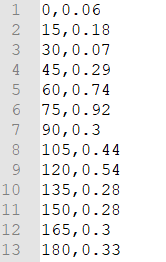
• Upload bar: the event is defined in a CSV file. The default format is in minutes, and the rainfall in mm for that time step. Please keep in mind that the duration of the rain in the custom format cannot exceed the duration of the simulation. Example of the format of a CSV file:

  

From NetCDF

• ‘The NetCDF contains:’ choose between time series of global values and raster time series (for spatially and temporally varying precipitation data).

• Upload bar: the event is defined in a NetCDF file. Use the processing algorithm Rasters to spatiotemporal NetCDF to generate such a file from a folder of tiffs. Please keep in mind that the duration of the rain in the custom format cannot exceed the duration of the simulation.

Design

• ‘Start after:’ defines an offset. The offset is the duration between start simulation and the start of the rainfall event.

• ‘Design number:’ a design number between 1 and 16 must be filled in. These numbers correlate to predetermined rain events, with differing return periods, that fall homogeneous over the entire model. Numbers 1 to 10 originate from RIONED and are heterogeneous in time. Numbers 11 to 16 have a constant rain intensity:

  Rain 11 statistically occurs once every 100 years. The duration of this event is 1 hour with a constant rain intensity of 70 mm/h. (T= 100.0 year, V=70 mm, Standard rain event (local) from Delta Programme 2019).

  Rain 12 statistically occurs once every 250 years. The duration of this event is 1 hour with a constant rain intensity of 90 mm/h. (T=250.0 year, V=90 mm, Standard rain event (local) from Delta Programme 2019).

  Rain 13 statistically occurs once every 1000 years. The duration of this event is 2 hours, with a constant rain intensity of 80 mm/h. (T=1000.0 year, V=160 mm, Standard rain event (local) from Delta Programme 2019).

  Rain 14 statistically occurs once every 100 years. The duration of this event is 48 hours, with a constant rain intensity of 2.5 mm/h. (T=100.0 year, V=120 mm, Standard rain event (regional) from Delta Programme 2019).

  Rain 15 statistically occurs once every 250 years. The duration of this event is 48 hours, with a constant rain intensity of 2.7 mm/h. (T=250.0 year, V=130 mm, Standard rain event (regional) from Delta Programme 2019).

  Rain 16 statistically occurs once every 1000 years. The duration of this event is 48 hours, with a constant rain intensity of 3.4 mm/h. (T=1000.0 year, V=160 mm, Standard rain event (regional) from Delta Programme 2019).

  These so-called design rain events are time series, which are traditionally used to test the functioning of a sewerage system in the Netherlands.

Radar - NL Only

This option is only available in the Netherlands and uses historical rainfall data that is based on radar rain images. Providing temporally and spatially varying rain information. The Dutch Nationale Regenradar is available for all Dutch applications. On request, the information from other radars can be made available to 3Di as well.

• ‘Start after:’ defines an offset. The offset is the duration between start simulation and the start of the rainfall event.

• ‘Stop after:’ the duration between the start of the simulation and the end of the rain event.

Note

Radar rain uses the time zone Central European Time. Make sure you select the same time zone for the start of your simulation on the Duration page to avoid confusion.

Wind

Wind in 3Di applies to 2D surface water. You can choose between a ‘Constant’ or a ‘Custom’ type of wind. Read more about wind and the physics used by 3Di here: Wind effects.

Constant

• ‘Start after:’ defining an offset for the drag coefficient. The offset is the duration between the start of the simulation and the start of the wind event.

• ‘Stop after:’ the duration between the start of the simulation and the end of the wind event.

• ‘Windspeed:’ the constant windspeed that will be added for the given time range (in m/s or km/h).

• ‘Drag coefficient:’ by increasing the drag coefficient, you increase the influence of the wind. It has a default value of 0,005.

• ‘Direction:’ the (meteorological) wind direction is defined as the direction from which the wind originates, measured in degrees clockwise from due north. Therefore, wind blowing toward the south has a direction of 0 degrees. You can either use the wind rose to depict which way the wind is blowing, or enter the direction manually.

Custom

• ‘Start after:’ defining an offset for the drag coefficient. The offset is the duration between the start of the simulation and the start of the wind event.

• ‘Drag coefficient:’ by increasing the drag coefficient, you increase the influence of the wind. It has a default value of 0,005.

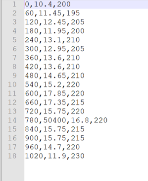
• ‘Values:’ upload a CSV in the format minutes, wind speed in m/s and wind direction, both for that time step.Here is and example of the format of a CSV file:

  

• the ‘Interpolate’ options will gradually change the wind speed or wind direction throughout a time series. Without the interpolate functions the wind speed and wind direction will stay constant within the time steps and will make an abrupt transition to the next time step.

Structure controls

Several structure properties can be changed during the simulation, such as the crest or gate level, pump capacity or discharge coefficients. These properties can be changed directly (using a timed control), or rules can be defined to let these properties react dynamically to changes in water level, volume, discharge, or flow velocity. See Structure control for more information.

From simulation template

When structure controls have been defined in the spatialite, this information will be read into the Simulation template when generating a 3Di Model. In the simulation wizard, the option ‘From simulation template’ will become available, so you can switch off some or all of the structure controls that are included in the simulation template.

Upload file

You can supply a JSON file that defines additional structure controls to be used in the simulation. If structure controls are already defined in the simulation template, the structure controls in the file will be added to those. The structure of the file is explained below. You can combine timed, table, and memory control in the same file.

Timed control

The following arguments can be specified for a Timed control:

Table 7 Arguments for a timed control

Name	Type	Units	Required	Description	Comments
offset	integer	seconds	Yes	Offset of event in simulation	-
duration	integer	seconds	Yes	Defines how long the control structure is active	-
value	decimal number	m MSL, -, m3/s	Yes	Structure property will be set to this value	Units depend on the type. Crest and gate levels in m MSL, discharge coefficients are unitless, pump capacities in m3/s.
type	string	-	Yes	Defines which structure property to set	Options are: ‘set_discharge_coefficients’, ‘set_crest_level’, ‘set_gate_level’, ‘set_pump_capacity’
structure_id	integer	-	No	ID of the structure as defined in the spatialite	Either structure_id or grid_id must be specified
structure_type	string	-	Yes	The type of structure that is to be controlled	Valid values: ‘v2_pumpstation’, ‘v2_pipe’, ‘v2_orifice’, ‘v2_culvert’, ‘v2_weir’, ‘v2_channel’
grid_id	integer	-	No	ID of the flowline or pump that is to be controlled	Either structure_id or grid_id must be specified

The value parameter must be a list, even if it contains 1 value (e.g. [0.3]), except for the set_discharge_coefficients action that expects a value for both flow directions (e.g. [0.8, 0.0]).

The following example JSON file sets the discharge coefficients of weir 21 to 0.4 (positive) and 0.8 (negative) for the first 100 s of the simulation:

{
    "timed": [
        {
          "offset": 0,
          "duration": 100,
          "value": [
            0.4, 0.8
          ],
          "type": "set_discharge_coefficients",
          "structure_id": 21,
          "structure_type": "v2_weir"
        }
    ]
}

Memory control

The following arguments can be specified for a Memory control:

Table 8 Arguments for a memory control

Name	Type	Units	Required	Description	Comments
offset	integer	seconds	Yes	Offset of event in simulation	-
duration	integer	seconds	Yes	Defines how long the control structure is active	-
measure_specification	Measure specification	-	Yes	Specifies how the value to which the control should react is measured	-
structure_id	integer	-	No	ID of the structure as defined in the spatialite	Either structure_id or grid_id must be specified
structure_type	string	-	Yes	The type of structure that is to be controlled	Valid values: ‘v2_pumpstation’, ‘v2_pipe’, ‘v2_orifice’, ‘v2_culvert’, ‘v2_weir’, ‘v2_channel’
type	string	-	Yes	Defines which structure property to set	Options are: ‘set_discharge_coefficients’, ‘set_crest_level’, ‘set_gate_level’, ‘set_pump_capacity’
value	list of decimal number(s)	m MSL, -, m3/s	Yes	Structure property will be set to this value	Units depend on the type. Crest and gate levels in m MSL, discharge coefficients are unitless, pump capacities in m3/s.
grid_id	integer	-	No	ID of the flowline or pump that is to be controlled	Either structure_id or grid_id must be specified
upper_threshold	decimal number	m MSL, m3, m/s, m3/s	No	-	-
lower_threshold	decimal number	m MSL, m3, m/s, m3/s	No	-	-
is_active	boolean	-	No	when True the initial state of the target is active	-
is_inverse	boolean	-	No	when True the target will become active when the lower threshold has been reached	-

The value parameter must be a list, even if it contains 1 value (e.g. [0.3]), except for the set_discharge_coefficients action that expects a value for both flow directions (e.g. [0.8, 0.0]).

The following example JSON file activates a memory control after one hour since the start of the simulation, that sets the crest level of weir 13 to 9.05 m MSL when the water level at connection node 356 rises above 0.3m. It will go back to its initial value when the water level falls below 0.1 m MSL:

{
    "memory": [
        {
          "offset": 3600,
          "duration": 259200,
          "measure_specification": {
            "locations": [
              {
                "weight": 1.00,
                "content_type": "v2_connection_node",
                "content_pk": 356
              }
            ],
            "variable": "s1",
            "operator": ">"
          },
          "structure_id": 13,
          "structure_type": "v2_weir",
          "type": "set_crest_level",
          "value": [
            9.05
          ],
          "upper_threshold": 0.3,
          "lower_threshold": 0.1,
          "is_active": false,
          "is_inverse": false
        }
    ]
}

Note

References to object types must include the v2_ prefix in this JSON file. This is a legacy of the table names in the schematisation database as defined up until March 2025 that has been upheld for reasons of backward compatibility.

The figure below shows three examples of JSON files.

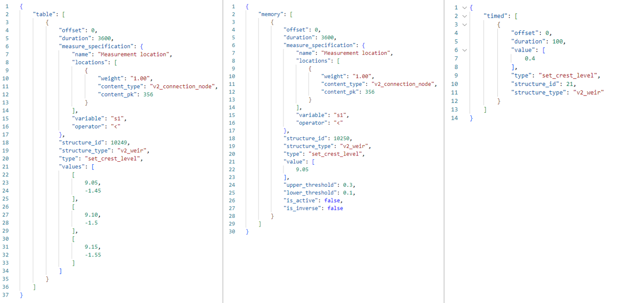
Table control

The following arguments can be specified for a Table control:

Table 9 Arguments for a table control

Name	Type	Units	Required	Description	Comments
offset	integer	seconds	Yes	Offset of event in simulation	-
duration	integer	seconds	Yes	Defines how long the control structure is active	-
measure_specification	Measure specification	-	Yes	Specifies how the value to which the control should react is measured	-
structure_id	integer	-	No	ID of the structure as defined in the spatialite	Either structure_id or grid_id must be specified
structure_type	string	-	Yes	The type of structure that is to be controlled	Valid values: ‘v2_pumpstation’, ‘v2_pipe’, ‘v2_orifice’, ‘v2_culvert’, ‘v2_weir’, ‘v2_channel’
type	string	-	Yes	Defines which structure property to set	Options are: ‘set_discharge_coefficients’, ‘set_crest_level’, ‘set_gate_level’, ‘set_pump_capacity’
values	list of decimal number(s)	m MSL, -, m3/s	Yes	See Values parameter of table control	-
grid_id	integer	-	No	ID of the flowline or pump that is to be controlled	Either structure_id or grid_id must be specified

The following example JSON file activates a table control during the first hour of the simulation. It that sets the gate level of orifice 27 to an action value defined in the action table, when the water level at connection node 356 falls below the threshold value in the action table:

{
    "table": [
        {
            "offset": 0,
            "duration": 3600,
            "measure_specification": {
                "locations": [
                    {
                        "weight": 1.00,
                        "content_type": "v2_connection_node",
                        "content_pk": 356
                    }
                ],
                "variable": "s1",
                "operator": "<"
            },
            "structure_id": 27,
            "structure_type": "v2_orifice",
            "type": "set_gate_level",
            "values": [
                [
                    9.05,
                    -1.45
                ],
                [
                    9.10,
                    -1.5
                ],
                [
                    9.15,
                    -1.55
                ]
            ]
        }
    ]
}

Note

References to object types must include the v2_ prefix in this JSON file. This is a legacy of the table names in the schematisation database as defined up until March 2025 that has been upheld for reasons of backward compatibility.

Values parameter of table control

The values parameter is an action table, which consists of one or more (threshold, action value) pairs, e.g. [[9.05, -1.45], [9.10, -1.5], [9.15, -1.55]]

To close/open or partially close/open a structure using the set_discharge_coefficients type, the values must contain three values. For example [[1.2, 0.5, 0.7]], where

• 1.2 is the threshold value

• 0.5 the action value for the positive flow direction

• 0.7 action value for the negative flow direction

Action values for set_discharge_coefficients type must be > 0.

For ALL operators threshold values must be ascending.

The units of the threshold values depend on the measure_specification. Water levels are in m MSL, volumes in m3, flow velocities in m/s, discharges in m3/s.

The units of the action values depend on the action type. Crest and gate levels in m MSL, discharge coefficients are unitless, pump capacities in m3/s.

Measure specification

A Measure specification defines how the value must be calculated that triggers a control structure action. It has the following parameters.

Table 10 Arguments for a control structure measure specification

Name	Type	Units	Required	Description	Comments
name	string	-	No	A name that describes this measure specification	-
locations	list of measure locations	-	Yes	-	-
variable	string	-	Yes	measurement variable, one of the following options: s1 (waterlevel), vol1 (volume), q (discharge), u1 (velocity)	-
operator	string	-	Yes	e.g. >, <, >=, <=	-

Measure location

A Measure location defines a location and its weight relative to other measure locations that are grouped in the same Measure specification. The sum of the weights for one Measure specification must equal 1. It is defined by the following arguments.

Table 11 Arguments for a control structure measure location

Name	Type	Required	Description
weight	decimal number	Yes	The weight to use for this location when calculating the weighted average of all measured values in their measure specification.
content_type	string	Yes	schematisation database table from which to select a feature to use as measure location, e.g. ‘v2_connection_node’
content_pk	integer	Yes	ID (primary key) of the feature to use as measure location.
grid_id	integer	No	Computational grid ID of the node or flowline to use as measure location.

Note

References to object types must include the v2_ prefix in this JSON file. This is a legacy of the table names in the schematisation database as defined up until March 2025 that has been upheld for reasons of backward compatibility.

Breaches

The dimension of a breach in a levee can be added to determine the flow through the breach and subsequently the flood. For a description on breaches, see: Breaches.

If you choose a model that incorporates breaches for simulation, a breaches file will be downloaded from the server and added to the layers panel when you select the desired model. The breaches will be visible in the map view. When adding a breach to your simulation the following parameters need to be filled in:

• ‘ID of breach:’ select the ID of the breach to be used in the simulation.

• ‘Initial width:’ specify the initial width of the breach.

• ‘Duration till max depth:’ determine the duration of the breach until it reaches its maximum depth.

• ‘Start after:’ defining an offset for the breach. The offset is the duration between the start of the simulation and the start of the breach event.

• ‘Max breach depth:’ set the maximum depth that the breach can reach.

• ‘Discharge coefficient positive/negative:’ these coefficients are utilized in the discharge formulation. Depending on the flow direction, the coefficients may vary.

Generate saved state after simulation

When you check this option the end result of the simulation will be saved as a saved state. A saved state file can be used as an initial condition. For more information, see: Saved states.

Post-processing in Lizard

Storing your results in Lizard and automated post-processing is only available for users of organisations with a Lizard account.

Checking the ‘Post-Processing in Lizard’ function will generate the following maps:

• water depth maps per output time step

• maximum water depth map for the whole simulation

• flood hazard rating

• rise velocity

• water level for each output time step

• maximum water level for the whole simulation

• max velocity

• rainfall

The Basic processed results are stored the 3Di output files in the Lizard platform:

• Result NetCDF (containing actual values)

• Aggregate NetCDF (availability and content dependent on user settings. required for water balance tool in Modeller Interface)

• Grid administration (gridadmin.h5 file. required to load NetCDF results in Modeller Interface)

• Calculation core logging (A zip containing logfiles)

All maps can be downloaded as GTiff, either via the interface https://demo.lizard.net/ or via the lizard API.

‘Arrival time map’: calculates a map showing the time of arrival of water per pixel in hours

‘Damage estimation’: automated estimate maps of damage as a result of flooding. This option takes into account water depth and duration of flood, resulting ing the following damage maps:

• Water depth (WSS)

• Damage (direct)

• Damage (indirect)

• Total damage

• And a damage summary in csv format. For more information check the documentation here: https://docs.lizard.net/e_catalog.html#results

Note

The damage estimations are only available in the Netherlands. Contact us at servicedesk@nelen-schuurmans.nl if you like to use this option and don’t have access yet.

Multiple simulations

This option becomes available when using either breaches or precipitation. You can define multiple simulations with different rainfall or breaches. Useful when simulating multiple events on the same model.