Checking the schematisation
It is highly recommended to check your schematisation before uploading. It helps you detect and solve errors or warnings early on.
Schematisation checker
The schematisation checker checks your 3Di schematisation (.gpkg file) for completeness and consistency between tables. It detects most database errors before uploading the schematisation to the 3Di servers for model generation.
In order to use the schematisation checker follow these steps:
Start the 3Di Modeller Interface
Open the processing algorithm in the 3Di Processing Algorithms > 3Di > Schematisation > Check Schematisation.
Choose to the geopackage file you want to check
Optionally, choose a location to store the outputs; otherwise, the output will be stored in a temporary file.
Click Run to run the schematisation checker. The outputs are added to your project as a table layer.
The output contains six columns: id, table, column, value, description and check:
id: identification number of the row where a check encounters an error.
table: the table in which the error occurs.
column: the column which contains the error.
value: the current value in the cell
description: description of the error
check: the type of check that found the error, described below
What is checked?
For a table of all the checks run on the schematisation, and their respective error codes, see the List of checks run by the schematisation checker on the schematisation.
Visualising computational grids
3Di builds a computational grid from schematisation data (stored in geopackage and rasters). This computational grid is stored in a “gridadmin.h5” file. You can visualize these grids in the 3Di Modeller Interface.
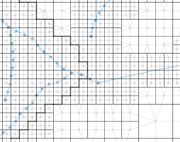
Fig. 10 An example of a visualised computational grid
You can also generate the computational grid from a schematisation. This is very useful to understand how the data in your schematisation is interpreted by 3Di. It answers questions like:
Is the data in the schematisation database valid, i.e. can a computational grid be created from it?
Where is each 2D cell located?
With which 2D cell does this channel exchange?
Which cell boundaries are affected by this obstacle?
Where are potential breaches located exactly?
Computational grid from gridadmin.h5 file
The processing algorithm “Computational grid from gridadmin.h5” reads the computational grid data from the .h5 file and writes it to GIS-layers in a GeoPackage. You can find it in the 3Di Processing Algorithms (Main Menu > Processing > Toolbox), under 3Di > Computational Grid. Choose a folder that contains a gridadmin.h5 file and an output location for the GeoPackage. Once the algorithm has run, the layers from the GeoPackage will be added to your project. If you do not need this data anymore after closing the 3Di Modeller Interface, you can also save to a temporary file.
Computational grid from schematisation
The processing algorithm “Computational grid from schematisation” builds a computational grid from schematisation data (stored in geopackage and rasters). The algorithm writes this to a gridadmin.h5 file and subsequently converts that data to GIS-layers in a GeoPackage. You can find it in the 3Di Processing Algorithms (Main Menu > Processing > Toolbox), under 3Di > Computational Grid. Choose your schematisation’s geopackage file and an output location for the GeoPackage. Once the algorithm has run, the layers from the GeoPackage will be added to your project. If you do not need this data anymore after closing the 3Di Modeller Interface, you can also save to a temporary file.
Differences between locally and server-generated grids
Please note that when generating the computational grid locally, some attributes will not be filled. The reason for this is that some information about the grid is generated by the routine that creates the volume tables (lookup tables that contain the relation between volume and water level, friction, etc.). This routine is run on the server, but not included in the grid building algorithm in the 3Di Modeller Interface. This applies to all attributes that are related to elevation in the 2D domain:
Node layer: max_surface_area, bottom_level (for 2D and embedded nodes). Also note that a node’s drain_level is only relevant if there is no 2D; otherwise, the exchange_level of the 1D flowline contains the relevant data.
Cell layer: max_surface_area, bottom_level, impervious_layer_elevation
Flowline layer: exchange_level (for 2D en 1D/2D flowlines)
Obstacles: exchange_level
Detecting leaking obstacles in the DEM
Two processing algorithms are available to help you identify leaking obstacles in the DEM, such as dikes or elevated roads in the dem that are ‘missed’ by 3Di because they do not cover the entire edge of a calculation cell. Access them via Main Menu > Processing > Toolbox > 3Di > Computational Grid.
Detect leaking obstacles in DEM analyses all 2D flowlines in the model domain.
Detect leaking obstacles in DEM (discharge threshold) analyses only the 2D flowlines in the model domain through which more than a specified volume of water flows during the entire simulation. It also estimates how much effect placing an obstacle would have on this volume.