Computational grid
To allow flow to be computed numerically, space and time must be discretised. Time steps are defined for time and grids are defined for space.
3Di models can consist of a 2D surface water, 2D groundwater and/or 1D network component. The surface water and groundwater components are a two-layer model, which can be coupled to the 1D network. The grids of the surface water and groundwater domain are similar, while the 1D network is fundamentally different. All these components are parts of one single grid, for which 3Di solves equations in a single matrix during the simulation.
In the sections below, we elaborate on the grids specified for computations in the 2D surface water and groundwater domains and in the 1D domain.
Computational grid for 2D domain
3Di uses a structured, staggered grid. For the 2D domain, this implies that computational cells are perfect squares. Pressure, water levels and volumes are defined in the cell centres; velocities and discharges are defined at the cell edges.
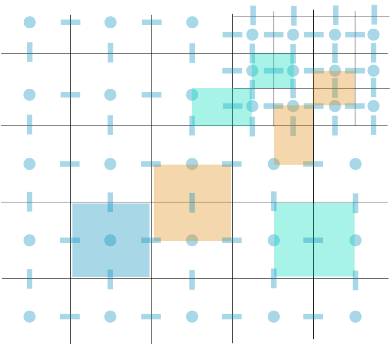
Fig. 42 Example of a staggered 2D grid including a refinement; water levels/ pressures are defined in the cell centres (blue dots) and velocities at the cell edges (blue bars). Water level domains are indicated by blue areas, and the momentum domains by green and orange areas.
The hydrodynamic computations are based on the conservation of volume and momentum. See Conservation of mass, 1D Flow, 2D Surface flow, and 2D Groundwater flow for more information. In order to solve these flow equations, the domains in which they are valid need to be defined first. In the Figure above, the volume and momentum domains are shown.
Grid refinement in 2D
The computational cost of a simulation is strongly related to the number of computational cells. One always needs to find a balance between grid resolution and computational time. In a model area, there are often regions in which flow is more complex or for which results with a finer resolution are required. To optimise the computational cost and grid resolution, users can refine the grid locally. 3Di uses a method called quad-tree refinement. The grid is refined subdividing cells in four; a cell edge can not be smaller less than half of its neighbour (see the Figure below). This is a simple refinement method that forces smooth grid variations, enhancing accurate solutions of the equations.
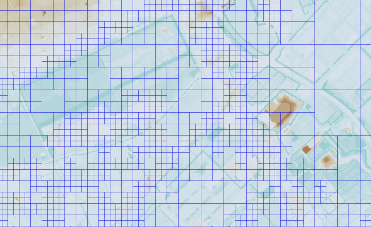
Fig. 43 An example of a computational grid with quad-tree refinements.
In models with groundwater, the grid refinement is applied in both the surface water layer and the groundwater layer.
2D grid settings
The 2D computational grid is generated based on the following settings: - Minimum cell size - Number of grid levels - Grid refinements
The Minimum cell size is the width or length of a computational cell. An even number of subgrid pixels must fit in the Minimum cell size. In case the dimensions of a subgrid pixel are 0.5 x 0.5 m2, the Minimum cell size can be 5.0 x 5.0 \(m^2\). In case the dimensions of a subgrid pixel are 1.0 x 1.0 m2, the Minimum cell size can not be 5.0 x 5.0 m2. The Minimum cell size is defined in the Model settings. The Number of grid levels setting is the number of refinement levels. Locations where the grid needs to be refined can be defined using a Grid refinement line, or a Grid refinement area. In case two refinement levels are defined at the same location, 3Di will refine to smallest cell size of the two. Next to the cells that intersect the grid refinement, the cells will become larger again. This is done using the quadtree method described above.
Note
A computational grid with many cell size transitions may also slow down the simulation. It is therefore recommended to merge grid refinements that are close together and prevent gaps between them. Sometimes a large area with uniform small cell size is more efficient than a large variation in cell sizes, even if the latter has fewer cells. Try out what works best in your situation.
Groundwater
For the groundwater domain, another 2D grid is used. This is coupled vertically with the grid for the surface domain. Again, pressure, water levels and volumes are defined in the cell centres while velocities and discharges are defined between vertically staggered cells. In the Figure below, an example of the two-layer coupling is shown.
Grid refinements are present in both the surface layer and the groundwater layer.
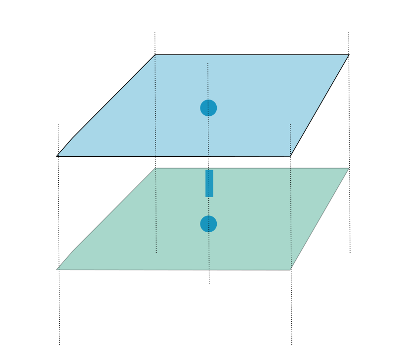
Fig. 44 Example of a vertically staggered grid.
Computational grid for 1D domain
In 3Di, 1D networks can be defined, representing open channels, manholes, weirs, orifices, culverts and closed pipes. This allows for an extensive description of the system, without actually computing cross-flow phenomena, reducing the computational cost.
There are several options to couple the 1D and the 2D domain (see Section 1D Flow). All options for the coupling allow for a fully integrated computation, which means that the full 1D and 2D systems are solved as one.
The 1D domain of the computational grid uses a staggered grid, just like the 2D domain (see the figure below). Volumes and water levels (or pressures) are defined at calculation nodes. Discharges and velocities are defined at velocity points in between the calculation nodes.
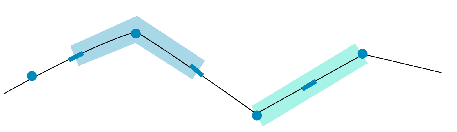
Fig. 45 An example of the grid of a 1D Network. Water levels (or pressures) are defined at the nodes (dark blue dots) and velocities at center of the flowline that connects the nodes (dark blue bars). Water level domains are indicated by the light blue areas, and the momentum domains by the light green areas.
Storage in the 1D domain
The available storage for a 1D node consists of the storage of the node (if the node is created at the location of a connection node that has a storage area > 0) plus the storage available in the halves of the channels, pipes, or culverts that connect to the node. This follows logically from the staggered grid approach. An example is given in the figure below.
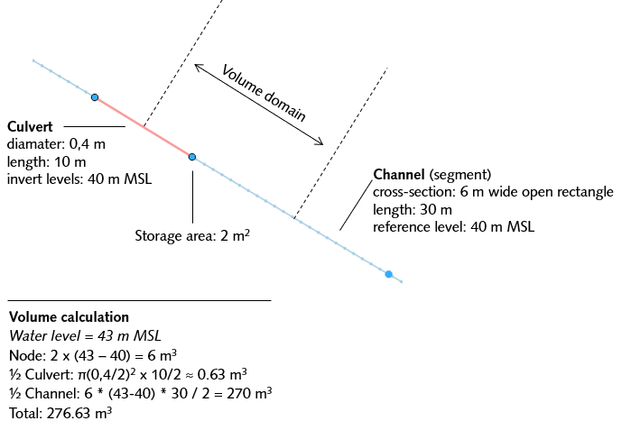
Fig. 46 Example of how storage is calculated in the 1D network: the volume in the node plus the half the volume of the culvert and channel that are connected to it.
Calculation point distance
When the computational grid is generated from the schematisation input, computational nodes are placed at each connection node. Additionally, computational nodes can be generated in between these locations. The spacing between these computational nodes is determined by a calculation point distance, the 1D grid resolution. In 3Di this distance can be specified for each individual pipe, culvert, or channel by filling the Calculation point distance attribute of those features. If the specified calculation point distance is larger than the length of the feature, no additional calculation nodes are generated in between the connection nodes. This is visualised in the figure below.
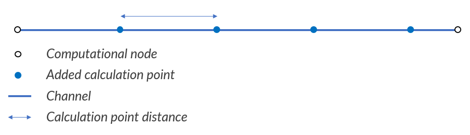
Fig. 47 Example of the generated calculation nodes between two nodes on a channel.
The cross-section of channel segments at a (new) velocity point is determined by linearly interpolating the wet cross-sectional area from the cross-section locations during the simulation. If a velocity point is not in between two cross-section locations, the cross-section from the nearest cross-section location is used. If more than two cross-section locations exist between two velocity points, the ones in the middle are ignored.
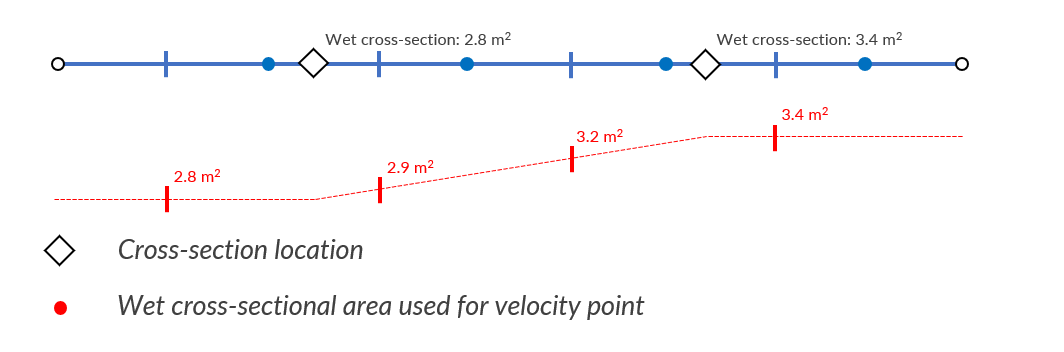
Fig. 48 Example of the generated velocity points between cross-section locations.
These additional computational nodes can have exchange types Isolated, (Double) connected or Embedded. This depends on the exchange type that was attributed to the original pipe, channel or culvert. In case of (double) connected elements, the exchange levels are set automatically. The exchange levels for for (double) connected elements are determined similarly as with the cross-sections. For channels, the bank levels for the additional computational nodes are determined by linear interpolation between the bank levels that are specified by the user at the cross-section locations on the channel. If the computational node is not in between two cross-section locations, the bank level of the nearest cross-section location is used. This is illustrated in the figure below. In case more than two cross-section locations are defined between two (new) computational nodes, the ones in the middle are ignored.
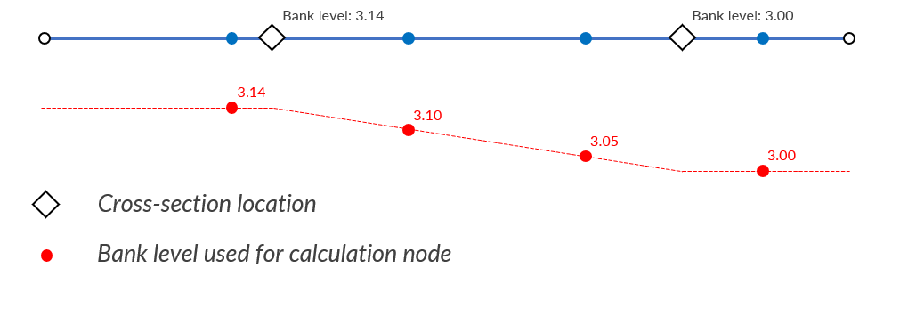
Fig. 49 Example of the used bank levels based on the cross-section locations for (double) connected elements.
For pipes and culverts, the drain level of the generated computational nodes is determined by linear interpolation between the drain levels at the start and end of the pipe or culvert. This is relevant only for pipes and culverts with exchange type Connected. In the case of pipes, this can be a way to schematise gullies. Pipes and culverts always have a single cross-section over their entire length, so interpolation of the cross-section is not necessary.
If drain levels are not set, the height of the DEM at that location is used as exchange height.
Computational grid objects
The computational grid can be visualised as vector layers). This section describes those vector layers and their attributes. The computational grid consists of the following objects:
Cell
Flowline
Node
Obstacle
Pump (line)
Pump (point)
Cell
The 2D cells (surface water and groundwater domains).
Geometry
Polygon
Attributes
Flowline
Line between two nodes
Geometry
Line.
Attributes
Attribute alias
Field name
Type
Units
Description
ID
id
integer
-
Unique identifier
Discharge coefficient positive
discharge_coefficient_positive
decimal number
-
Discharge coefficient in the positive direction.
Discharge coefficient negative
discharge_coefficient_negative
decimal number
-
Discharge coefficient in the negative direction.
Line type
line_type
integer
-
Flowline type, e.g. 2D, 1D connected or 1D isolated
Source table
source_table
text
-
Name of the layer in the schematisation database from which this flowline was generated.
Source table ID
source_table_id
integer
-
The ID of the feature in the schematisation database layer from which this flowline was generated.
Invert level of the start point
invert_level_start_point
decimal number
m MSL
Invert level of the start point of the object.
Invert level of the end point
invert_level_end_point
decimal number
m MSL
Invert level of the end point of the object.
Exchange level
exchange_level
decimal number
m MSL
Water only flows through this flowline if the water level in either the start node or the end node exceeds the exchange level.
Start calculation node ID
calculation_node_id_start
integer
-
ID of the calculation node at the start of the flowline.
End calculation node ID
calculation_node_id_end
integer
-
ID of the calculation node at the end of the flowline.
Sewerage
sewerage
boolean
-
True if flowline belongs to a sewerage object. Used for visualisation and administrative purposes only.
Sewerage type
sewerage_type
integer
-
Function of the pipe in the sewerage system. Used for visualisation and administrative purposes only. See Notes for modellers.
Node
Node in the computational grid where volumes and water levels are defined. In the 2D domain, the node is located at the center of a cell.
Geometry
Point.
Attributes
Attribute alias
Field name
Type
Units
Description
ID
id
integer
-
Unique identifier
Connection node ID
connection_node_id
integer
-
If applicable: ID of the connection node from which this calculation node was generated.
Node type
node_type
integer
-
Defines the type of the calculation node as 2D Surface water (1), 2D Groundwater (2), 1D open water (3), 1D closed system (4), 2D Surface water boundary (5), 2D Groundwater boundary (6), or 1D Boundary (7).
Calculation type
calculation_type
integer
Yes
-
1D2D exchange type: embedded (0), isolated (1), connected (2), or double connected (5). See Exchange types.
Is manhole
is_manhole
boolean
-
True if the bottom level was filled in for the connection node from which this node was generated
Storage area of the connection node
connection_node_storage_area
decimal number
m2
-
Maximum surface area
max_surface_area
decimal number
m2
Largest possible wet surface area for this node
Bottom level
bottom_level
decimal number
m MSL
Lowest point of this node
Drain level
drain_level
decimal number
m MSL
Exchange level that was filled in for the connection node form which this node was generated. Drain level of the manhole. See also notes_for_modellers_connection_nodes_exchange_level.
Obstacle
Border of a computational cell that was affected by an obstacle. The exchange level of intersected flowlines may be affected by this obstacle (depending on the obstacle’s settings).
Geometry
Line.
Attributes
Attribute alias
Field name
Type
Units
Description
ID
line_id
integer
-
Unique identifier
Exchange level
exchange_level
decimal number
m MSL
Exchange level for the obstacle.
Pump (line)
Pump that transports water from one connection node to another.
Geometry
Line.
Attributes
Attribute alias
Field name
Type
Units
Description
ID
id
integer
-
Unique identifier
Display name
display_name
text
-
Name field
Start calculation node ID
calculation_node_id_start
integer
-
ID of calculation node from which the water is pumped.
End calculation node ID
calculation_node_id_end
integer
-
ID of calculation node to which the water is pumped.
Source table ID
source_table_id
integer
-
ID of the feature in the Pump layer in the schematisation database from which this pump is generated.
Type
type
integer
-
Sets whether pump reacts to water level at: suction side (1) or delivery side (2).
Bottom level
bottom_level
decimal number
m MSL
Lowest point of the node from which the water is pumped.
Start level
start_level
decimal number
Yes
m MSL
Pump switches on when the water level exceeds this level.
Lower stop level
lower_stop_level
decimal number
Yes
m MSL
Pump switches off when the water level becomes lower than this level.
Capacity
capacity
decimal number
Yes
L/s
Pump capacity.
Pump (point)
Pump that pumps water out of the model domain or to another calculation node within the model.
Geometry
Point.
Attributes
Attribute alias
Field name
Type
Units
Description
ID
id
integer
-
Unique identifier
Display name
display_name
text
-
Name field
Start calculation node ID
calculation_node_id_start
integer
-
ID of calculation node from which the water is pumped.
End calculation node ID
calculation_node_id_end
integer
-
ID of calculation node to which the water is pumped.
Source table ID
source_table_id
integer
-
ID of the feature in the Pump layer in the schematisation database from which this pump is generated.
Type
type
integer
-
Sets whether pump reacts to water level at: suction side (1) or delivery side (2).
Bottom level
bottom_level
decimal number
m MSL
Lowest point of the node from which the water is pumped.
Start level
start_level
decimal number
Yes
m MSL
Pump switches on when the water level exceeds this level.
Lower stop level
lower_stop_level
decimal number
Yes
m MSL
Pump switches off when the water level becomes lower than this level.
Capacity
capacity
decimal number
Yes
L/s
Pump capacity.